Easy Graph for Precision Recall F1 and Support Python

How to Calculate Precision, Recall, F1, and More for Deep Learning Models

Last Updated on August 27, 2020

Once you fit a deep learning neural network model, you must evaluate its performance on a test dataset.

This is critical, as the reported performance allows you to both choose between candidate models and to communicate to stakeholders about how good the model is at solving the problem.

The Keras deep learning API model is very limited in terms of the metrics that you can use to report the model performance.

I am frequently asked questions, such as:

How can I calculate the precision and recall for my model?

And:

How can I calculate the F1-score or confusion matrix for my model?

In this tutorial, you will discover how to calculate metrics to evaluate your deep learning neural network model with a step-by-step example.

After completing this tutorial, you will know:

• How to use the scikit-learn metrics API to evaluate a deep learning model.
• How to make both class and probability predictions with a final model required by the scikit-learn API.
• How to calculate precision, recall, F1-score, ROC AUC, and more with the scikit-learn API for a model.

Kick-start your project with my new book Deep Learning With Python, including step-by-step tutorials and the Python source code files for all examples.

Let's get started.

• Update Jan/2020: Updated API for Keras 2.3 and TensorFlow 2.0.

How to Calculate Precision, Recall, F1, and More for Deep Learning Models
Photo by John, some rights reserved.

Tutorial Overview

This tutorial is divided into three parts; they are:

1. Binary Classification Problem
2. Multilayer Perceptron Model
3. How to Calculate Model Metrics

Binary Classification Problem

We will use a standard binary classification problem as the basis for this tutorial, called the "two circles" problem.

It is called the two circles problem because the problem is comprised of points that when plotted, show two concentric circles, one for each class. As such, this is an example of a binary classification problem. The problem has two inputs that can be interpreted as x and y coordinates on a graph. Each point belongs to either the inner or outer circle.

The make_circles() function in the scikit-learn library allows you to generate samples from the two circles problem. The "n_samples" argument allows you to specify the number of samples to generate, divided evenly between the two classes. The "noise" argument allows you to specify how much random statistical noise is added to the inputs or coordinates of each point, making the classification task more challenging. The "random_state" argument specifies the seed for the pseudorandom number generator, ensuring that the same samples are generated each time the code is run.

The example below generates 1,000 samples, with 0.1 statistical noise and a seed of 1.

# generate 2d classification dataset X , y = make_circles ( n_samples = 1000 , noise = 0.1 , random_state = 1 )

Once generated, we can create a plot of the dataset to get an idea of how challenging the classification task is.

The example below generates samples and plots them, coloring each point according to the class, where points belonging to class 0 (outer circle) are colored blue and points that belong to class 1 (inner circle) are colored orange.

# Example of generating samples from the two circle problem from sklearn . datasets import make_circles from matplotlib import pyplot from numpy import where # generate 2d classification dataset X , y = make_circles ( n_samples = 1000 , noise = 0.1 , random_state = 1 ) # scatter plot, dots colored by class value for i in range ( 2 ) : samples_ix = where ( y == i ) pyplot . scatter ( X [ samples_ix , 0 ] , X [ samples_ix , 1 ] ) pyplot . show ( )

Running the example generates the dataset and plots the points on a graph, clearly showing two concentric circles for points belonging to class 0 and class 1.

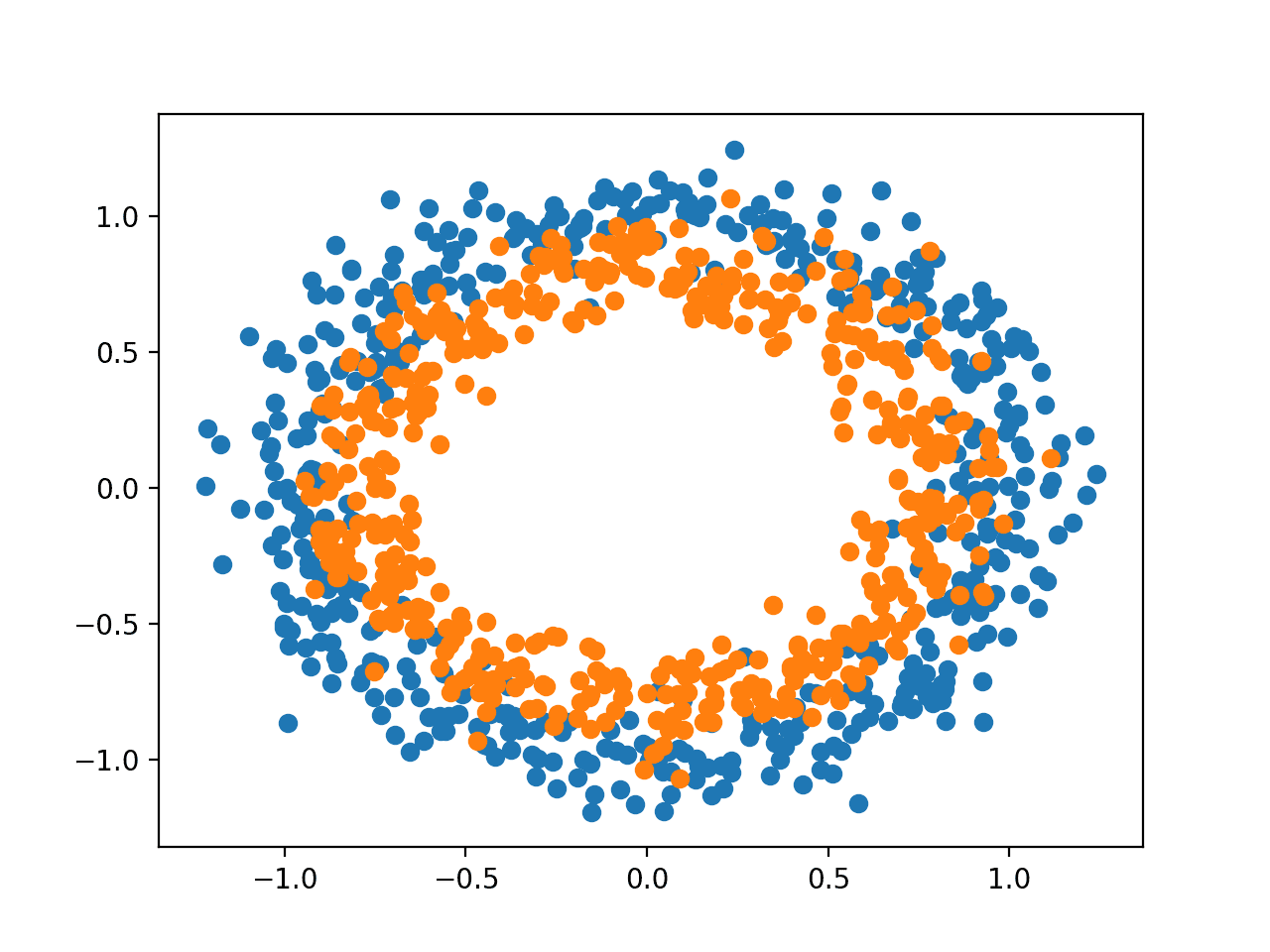
Scatter Plot of Samples From the Two Circles Problem

Multilayer Perceptron Model

We will develop a Multilayer Perceptron, or MLP, model to address the binary classification problem.

This model is not optimized for the problem, but it is skillful (better than random).

After the samples for the dataset are generated, we will split them into two equal parts: one for training the model and one for evaluating the trained model.

# split into train and test n_test = 500 trainX , testX = X [ : n_test , : ] , X [ n_test : , : ] trainy , testy = y [ : n_test ] , y [ n_test : ]

Next, we can define our MLP model. The model is simple, expecting 2 input variables from the dataset, a single hidden layer with 100 nodes, and a ReLU activation function, then an output layer with a single node and a sigmoid activation function.

The model will predict a value between 0 and 1 that will be interpreted as to whether the input example belongs to class 0 or class 1.

# define model model = Sequential ( ) model . add ( Dense ( 100 , input_dim = 2 , activation = 'relu' ) ) model . add ( Dense ( 1 , activation = 'sigmoid' ) )

The model will be fit using the binary cross entropy loss function and we will use the efficient Adam version of stochastic gradient descent. The model will also monitor the classification accuracy metric.

# compile model model . compile ( loss = 'binary_crossentropy' , optimizer = 'adam' , metrics = [ 'accuracy' ] )

We will fit the model for 300 training epochs with the default batch size of 32 samples and evaluate the performance of the model at the end of each training epoch on the test dataset.

# fit model history = model . fit ( trainX , trainy , validation_data = ( testX , testy ) , epochs = 300 , verbose = 0 )

At the end of training, we will evaluate the final model once more on the train and test datasets and report the classification accuracy.

# evaluate the model _ , train_acc = model . evaluate ( trainX , trainy , verbose = 0 ) _ , test_acc = model . evaluate ( testX , testy , verbose = 0 )

Finally, the performance of the model on the train and test sets recorded during training will be graphed using a line plot, one for each of the loss and the classification accuracy.

# plot loss during training pyplot . subplot ( 211 ) pyplot . title ( 'Loss' ) pyplot . plot ( history . history [ 'loss' ] , label = 'train' ) pyplot . plot ( history . history [ 'val_loss' ] , label = 'test' ) pyplot . legend ( ) # plot accuracy during training pyplot . subplot ( 212 ) pyplot . title ( 'Accuracy' ) pyplot . plot ( history . history [ 'accuracy' ] , label = 'train' ) pyplot . plot ( history . history [ 'val_accuracy' ] , label = 'test' ) pyplot . legend ( ) pyplot . show ( )

Tying all of these elements together, the complete code listing of training and evaluating an MLP on the two circles problem is listed below.

1 2 3 4 5 6 7 8 9 10 11 12 13 14 15 16 17 18 19 20 21 22 23 24 25 26 27 28 29 30 31 32 33 34 35 36

# multilayer perceptron model for the two circles problem from sklearn . datasets import make_circles from keras . models import Sequential from keras . layers import Dense from matplotlib import pyplot # generate dataset X , y = make_circles ( n_samples = 1000 , noise = 0.1 , random_state = 1 ) # split into train and test n_test = 500 trainX , testX = X [ : n_test , : ] , X [ n_test : , : ] trainy , testy = y [ : n_test ] , y [ n_test : ] # define model model = Sequential ( ) model . add ( Dense ( 100 , input_dim = 2 , activation = 'relu' ) ) model . add ( Dense ( 1 , activation = 'sigmoid' ) ) # compile model model . compile ( loss = 'binary_crossentropy' , optimizer = 'adam' , metrics = [ 'accuracy' ] ) # fit model history = model . fit ( trainX , trainy , validation_data = ( testX , testy ) , epochs = 300 , verbose = 0 ) # evaluate the model _ , train_acc = model . evaluate ( trainX , trainy , verbose = 0 ) _ , test_acc = model . evaluate ( testX , testy , verbose = 0 ) print ( 'Train: %.3f, Test: %.3f' % ( train_acc , test_acc ) ) # plot loss during training pyplot . subplot ( 211 ) pyplot . title ( 'Loss' ) pyplot . plot ( history . history [ 'loss' ] , label = 'train' ) pyplot . plot ( history . history [ 'val_loss' ] , label = 'test' ) pyplot . legend ( ) # plot accuracy during training pyplot . subplot ( 212 ) pyplot . title ( 'Accuracy' ) pyplot . plot ( history . history [ 'accuracy' ] , label = 'train' ) pyplot . plot ( history . history [ 'val_accuracy' ] , label = 'test' ) pyplot . legend ( ) pyplot . show ( )

Running the example fits the model very quickly on the CPU (no GPU is required).

Note: Your results may vary given the stochastic nature of the algorithm or evaluation procedure, or differences in numerical precision. Consider running the example a few times and compare the average outcome.

The model is evaluated, reporting the classification accuracy on the train and test sets of about 83% and 85% respectively.

Train: 0.838, Test: 0.850

A figure is created showing two line plots: one for the learning curves of the loss on the train and test sets and one for the classification on the train and test sets.

The plots suggest that the model has a good fit on the problem.

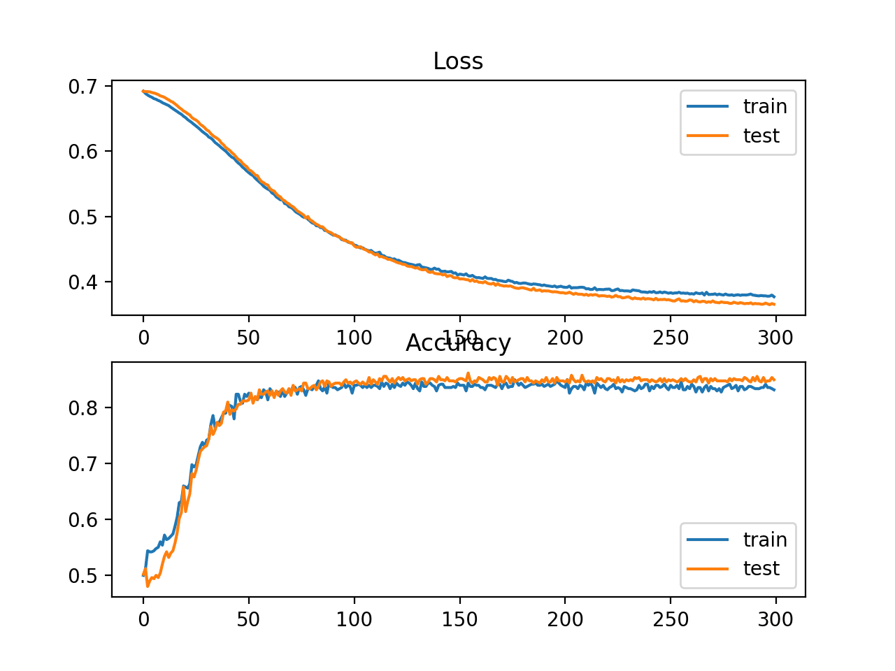
Line Plot Showing Learning Curves of Loss and Accuracy of the MLP on the Two Circles Problem During Training

How to Calculate Model Metrics

Perhaps you need to evaluate your deep learning neural network model using additional metrics that are not supported by the Keras metrics API.

The Keras metrics API is limited and you may want to calculate metrics such as precision, recall, F1, and more.

One approach to calculating new metrics is to implement them yourself in the Keras API and have Keras calculate them for you during model training and during model evaluation.

For help with this approach, see the tutorial:

• How to Use Metrics for Deep Learning With Keras in Python

This can be technically challenging.

A much simpler alternative is to use your final model to make a prediction for the test dataset, then calculate any metric you wish using the scikit-learn metrics API.

Three metrics, in addition to classification accuracy, that are commonly required for a neural network model on a binary classification problem are:

• Precision
• Recall
• F1 Score

In this section, we will calculate these three metrics, as well as classification accuracy using the scikit-learn metrics API, and we will also calculate three additional metrics that are less common but may be useful. They are:

• Cohen's Kappa
• ROC AUC
• Confusion Matrix.

This is not a complete list of metrics for classification models supported by scikit-learn; nevertheless, calculating these metrics will show you how to calculate any metrics you may require using the scikit-learn API.

For a full list of supported metrics, see:

• sklearn.metrics: Metrics API
• Classification Metrics Guide

The example in this section will calculate metrics for an MLP model, but the same code for calculating metrics can be used for other models, such as RNNs and CNNs.

We can use the same code from the previous sections for preparing the dataset, as well as defining and fitting the model. To make the example simpler, we will put the code for these steps into simple function.

First, we can define a function called get_data() that will generate the dataset and split it into train and test sets.

# generate and prepare the dataset def get_data ( ) : # generate dataset X , y = make_circles ( n_samples = 1000 , noise = 0.1 , random_state = 1 ) # split into train and test n_test = 500 trainX , testX = X [ : n_test , : ] , X [ n_test : , : ] trainy , testy = y [ : n_test ] , y [ n_test : ] return trainX , trainy , testX , testy

Next, we will define a function called get_model() that will define the MLP model and fit it on the training dataset.

# define and fit the model def get_model ( trainX , trainy ) : # define model model = Sequential ( ) model . add ( Dense ( 100 , input_dim = 2 , activation = 'relu' ) ) model . add ( Dense ( 1 , activation = 'sigmoid' ) ) # compile model model . compile ( loss = 'binary_crossentropy' , optimizer = 'adam' , metrics = [ 'accuracy' ] ) # fit model model . fit ( trainX , trainy , epochs = 300 , verbose = 0 ) return model

We can then call the get_data() function to prepare the dataset and the get_model() function to fit and return the model.

# generate data trainX , trainy , testX , testy = get_data ( ) # fit model model = get_model ( trainX , trainy )

Now that we have a model fit on the training dataset, we can evaluate it using metrics from the scikit-learn metrics API.

First, we must use the model to make predictions. Most of the metric functions require a comparison between the true class values (e.g. testy) and the predicted class values (yhat_classes). We can predict the class values directly with our model using the predict_classes() function on the model.

Some metrics, like the ROC AUC, require a prediction of class probabilities (yhat_probs). These can be retrieved by calling the predict() function on the model.

For more help with making predictions using a Keras model, see the post:

• How to Make Predictions With Keras

We can make the class and probability predictions with the model.

# predict probabilities for test set yhat_probs = model . predict ( testX , verbose = 0 ) # predict crisp classes for test set yhat_classes = model . predict_classes ( testX , verbose = 0 )

The predictions are returned in a two-dimensional array, with one row for each example in the test dataset and one column for the prediction.

The scikit-learn metrics API expects a 1D array of actual and predicted values for comparison, therefore, we must reduce the 2D prediction arrays to 1D arrays.

# reduce to 1d array yhat_probs = yhat_probs [ : , 0 ] yhat_classes = yhat_classes [ : , 0 ]

We are now ready to calculate metrics for our deep learning neural network model. We can start by calculating the classification accuracy, precision, recall, and F1 scores.

# accuracy: (tp + tn) / (p + n) accuracy = accuracy_score ( testy , yhat_classes ) print ( 'Accuracy: %f' % accuracy ) # precision tp / (tp + fp) precision = precision_score ( testy , yhat_classes ) print ( 'Precision: %f' % precision ) # recall: tp / (tp + fn) recall = recall_score ( testy , yhat_classes ) print ( 'Recall: %f' % recall ) # f1: 2 tp / (2 tp + fp + fn) f1 = f1_score ( testy , yhat_classes ) print ( 'F1 score: %f' % f1 )

Notice that calculating a metric is as simple as choosing the metric that interests us and calling the function passing in the true class values (testy) and the predicted class values (yhat_classes).

We can also calculate some additional metrics, such as the Cohen's kappa, ROC AUC, and confusion matrix.

Notice that the ROC AUC requires the predicted class probabilities (yhat_probs) as an argument instead of the predicted classes (yhat_classes).

# kappa kappa = cohen_kappa_score ( testy , yhat_classes ) print ( 'Cohens kappa: %f' % kappa ) # ROC AUC auc = roc_auc_score ( testy , yhat_probs ) print ( 'ROC AUC: %f' % auc ) # confusion matrix matrix = confusion_matrix ( testy , yhat_classes ) print ( matrix )

Now that we know how to calculate metrics for a deep learning neural network using the scikit-learn API, we can tie all of these elements together into a complete example, listed below.

1 2 3 4 5 6 7 8 9 10 11 12 13 14 15 16 17 18 19 20 21 22 23 24 25 26 27 28 29 30 31 32 33 34 35 36 37 38 39 40 41 42 43 44 45 46 47 48 49 50 51 52 53 54 55 56 57 58 59 60 61 62 63 64 65 66 67 68 69 70

# demonstration of calculating metrics for a neural network model using sklearn from sklearn . datasets import make_circles from sklearn . metrics import accuracy_score from sklearn . metrics import precision_score from sklearn . metrics import recall_score from sklearn . metrics import f1_score from sklearn . metrics import cohen_kappa_score from sklearn . metrics import roc_auc_score from sklearn . metrics import confusion_matrix from keras . models import Sequential from keras . layers import Dense # generate and prepare the dataset def get_data ( ) : # generate dataset X , y = make_circles ( n_samples = 1000 , noise = 0.1 , random_state = 1 ) # split into train and test n_test = 500 trainX , testX = X [ : n_test , : ] , X [ n_test : , : ] trainy , testy = y [ : n_test ] , y [ n_test : ] return trainX , trainy , testX , testy # define and fit the model def get_model ( trainX , trainy ) : # define model model = Sequential ( ) model . add ( Dense ( 100 , input_dim = 2 , activation = 'relu' ) ) model . add ( Dense ( 1 , activation = 'sigmoid' ) ) # compile model model . compile ( loss = 'binary_crossentropy' , optimizer = 'adam' , metrics = [ 'accuracy' ] ) # fit model model . fit ( trainX , trainy , epochs = 300 , verbose = 0 ) return model # generate data trainX , trainy , testX , testy = get_data ( ) # fit model model = get_model ( trainX , trainy ) # predict probabilities for test set yhat_probs = model . predict ( testX , verbose = 0 ) # predict crisp classes for test set yhat_classes = model . predict_classes ( testX , verbose = 0 ) # reduce to 1d array yhat_probs = yhat_probs [ : , 0 ] yhat_classes = yhat_classes [ : , 0 ] # accuracy: (tp + tn) / (p + n) accuracy = accuracy_score ( testy , yhat_classes ) print ( 'Accuracy: %f' % accuracy ) # precision tp / (tp + fp) precision = precision_score ( testy , yhat_classes ) print ( 'Precision: %f' % precision ) # recall: tp / (tp + fn) recall = recall_score ( testy , yhat_classes ) print ( 'Recall: %f' % recall ) # f1: 2 tp / (2 tp + fp + fn) f1 = f1_score ( testy , yhat_classes ) print ( 'F1 score: %f' % f1 ) # kappa kappa = cohen_kappa_score ( testy , yhat_classes ) print ( 'Cohens kappa: %f' % kappa ) # ROC AUC auc = roc_auc_score ( testy , yhat_probs ) print ( 'ROC AUC: %f' % auc ) # confusion matrix matrix = confusion_matrix ( testy , yhat_classes ) print ( matrix )

Note: Your results may vary given the stochastic nature of the algorithm or evaluation procedure, or differences in numerical precision. Consider running the example a few times and compare the average outcome.

Running the example prepares the dataset, fits the model, then calculates and reports the metrics for the model evaluated on the test dataset.

Accuracy: 0.842000 Precision: 0.836576 Recall: 0.853175 F1 score: 0.844794 Cohens kappa: 0.683929 ROC AUC: 0.923739 [[206  42] [ 37 215]]

If you need help interpreting a given metric, perhaps start with the "Classification Metrics Guide" in the scikit-learn API documentation: Classification Metrics Guide

Also, checkout the Wikipedia page for your metric; for example: Precision and recall, Wikipedia.

Further Reading

This section provides more resources on the topic if you are looking to go deeper.

Posts

• How to Use Metrics for Deep Learning With Keras in Python
• How to Generate Test Datasets in Python With scikit-learn
• How to Make Predictions With Keras

API

• sklearn.metrics: Metrics API
• Classification Metrics Guide
• Keras Metrics API
• sklearn.datasets.make_circles API

Articles

• Evaluation of binary classifiers, Wikipedia.
• Confusion Matrix, Wikipedia.
• Precision and recall, Wikipedia.

Summary

In this tutorial, you discovered how to calculate metrics to evaluate your deep learning neural network model with a step-by-step example.

Specifically, you learned:

• How to use the scikit-learn metrics API to evaluate a deep learning model.
• How to make both class and probability predictions with a final model required by the scikit-learn API.
• How to calculate precision, recall, F1-score, ROC, AUC, and more with the scikit-learn API for a model.

Do you have any questions?
Ask your questions in the comments below and I will do my best to answer.

Develop Deep Learning Projects with Python!

 What If You Could Develop A Network in Minutes

...with just a few lines of Python

Discover how in my new Ebook:
Deep Learning With Python

It covers end-to-end projects on topics like:
Multilayer Perceptrons,Convolutional Nets andRecurrent Neural Nets, and more...

Finally Bring Deep Learning To
Your Own Projects

Skip the Academics. Just Results.

See What's Inside

monniercyruch.blogspot.com

Source: https://machinelearningmastery.com/how-to-calculate-precision-recall-f1-and-more-for-deep-learning-models/

Share this post